Object-Dependent Surface Elements Data

To display the properties of all surface elements of any given object, select View | Surface Elements Data. This will allow data to be displayed in the form of:

• a table
• a color contour plot
• statistical data for an object.

Data is displayed for one target component at a time. The target component is selected using the drop-down box at the top of the dialog. For target components with a non-zero thickness -- i.e., they are composed of a outer (or top) wall and an inner (or bottom) wall -- data for only one of the walls is shown at a time.

Viewing Table Data

Initially, a table is displayed showing the following quantities:

• position of the surface element's centroid, displayed in the coordinate system of the target component
• surface index
• emission temperature
• radiation temperature
• radiation flux incident on the surface element
• radiation flux emitted by the surface element
• power source term (if due to incident laser beam, this includes correction for x-ray conversion efficiency)
• total laser power deposited
• albedo
• x-ray conversion efficiency
• laser reflectivity
• laser power deposited directly by beams
• laser power deposited by short-pulse beams due to portion of beam prior to reflection off of OAPs
• laser power deposited due to all reflections (glint)
• laser power deposited by individual reflections

The deviation from the mean value (averaged over an object) for individual surface elements can be displayed in table form in the Surface Element Properties widget. This is done by selecting Deviation from mean in the combo box at the top of the table.

In addition to specifying the Target Component, the user specifies the Wall Type. The wall type is used to specify which surface elements of the object to show (e.g., either the Front or Back portion of a cylinder that has a finite (non-zero) wall thickness; or the LEH at the top of a cylindrical hohlraum). The choice of Wall Type affects which surfaces elements are shown both in the table and the contour plots.

Surface element centroid positions are displayed in the coordinate system of the target component. The coordinates displayed depend of the type of target component [e.g., (r,θ,φ) for spherical objects, (r,θ,z) for cylindrical objects, etc.]. Note that viewing the position of surface elements in the target chamber coordinate system can be done for individual surface elements (see Results for individual surface elements).

Note that the centroid positions for surface elements of objects with curved surfaces may have radii slightly different from the radii entered in the size-grid tab of the Object Parameters Dialog. This can occur because: (1) objects are composed of surfaces with flat polygons, and (2) the node positions of object grids are normalized such that the total surface area of each object is consistent with parameters entered in the Object Parameters Dialog.

The Columns button allows the user to show or hide table columns.

The Refresh buttons updates values in the table in the event that data has changed.

Surface element data can be dumped to multi-column ascii files using File menu items:

Viewing Color Contours

Color contour plots can be generated for individual objects. Graphs are displayed in the natural coordinate system of the object (e.g., for a sphere, quantities are plotted vs. polar angle and azimuthal angle). Quantities that can be displayed include:

• Emission temperature
• Radiation temperature
• Radiation flux incident
• Radiation flux emitted
• Power source term (if due to incident laser beam, this includes correction for x-ray conversion efficiency)
• Total laser power deposited (includes direct and reflected laser light)
• Direct laser power deposited
• Direct laser power deposited for a single beam cone
• Laser power deposited due to all reflections (glint)

To display a contour plot, select Plot | <quantity> using the menu bar on the Surface Element Properties widget.

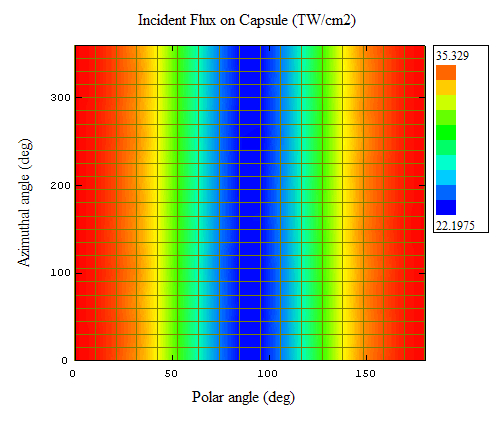
The intersection points of laser beam cones with the object being examined can be shown on the contour plot. To do this, select Beam Spots | Show from the menu at the top of the contour plotter.

• The beam spot color can be changed using the Beam Spots | Set Spots Color menu item.
• The beam spot label attributes can be changed by selecting one or more beam spot labels, and right-clicking with the mouse to display options for editing.
• The beam spot labels can be re-generated (which resets the label text, fonts, colors, and positions) using the Beam Spots | Regenerate Labels menu item.
• The beam spot labels can be reset to their default locations, without changing the text, fonts, or colors, using the Beam Spots | Reset Label Positions menu item.

Contour plots for Sphere objects can also be shown using sinusoidal projection (i.e., Hammer-Aitoff projection), such as in the example below. To do this, select select View | Plot Type | Sinusoidal from the menu at the top of the contour plotter.

Lineout displays can be accessed by Lineout Tool Button () at the top of the Surface Element Properties widget. Lineouts can be generated along the horizontal and vertical directions (see example below). The cross hairs in the color contour plot are used to specify the horizontal and vertical lineout positions.

Viewing Statistical Data for Objects

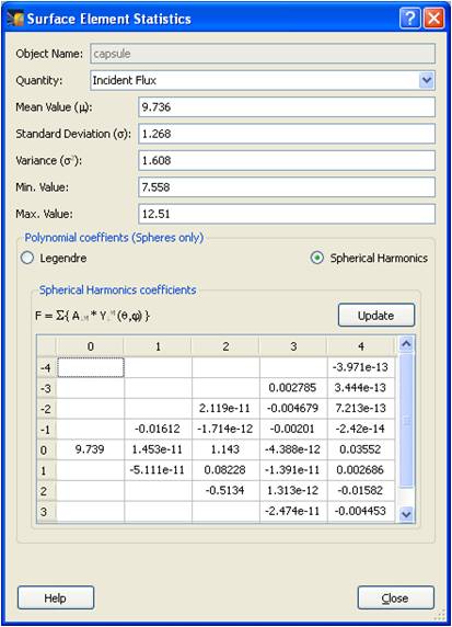
Statistical data can be displayed for individual objects. Quantities available are the same as listed above (radiation temperature, etc.). Statistical data include:

• mean
• variance
• standard deviation
• minimum value
• maximum value.

Statistical data are accessed through the Analysis menu on the Surface Element Properties widget.

The deviation from the mean value (averaged over an object) for individual surface elements can be displayed in table form in the Surface Element Properties widget. This is done by selecting Deviation from mean in the combo box at the top of the table.

When viewing data for Sphere objects, best fit values for Legendre polynomial coefficients and Spherical Harmonics coefficients can also be displayed in the Surface Element Statistics widget. Fits to Legendre and Spherical Harmonics coefficients are supported for the following quantities:

• Incident radiation flux
• Total laser power deposited
• Direct laser power deposited.

Legendre coefficients are fitted to the expression:

Flux (θ) = A₀ + A₁ P₁(cos(θ)) + A₂ P₂(cos(θ)) + A₃ P₃(cos(θ)) + A₄ P₄(cos(θ))

where A_n are fitting coefficients and P_n are Legendre polynomials. Coefficients used in the fitting expansion range up through A₄, and are selected by checking the appropriate check boxes.  To update the fitting after selecting/deselecting coefficients, hit the Update button.

Spherical harmonics coefficients are fitted to the expression:

Flux (θ,φ) = Σ_LM  ( A_LM Y_LM (θ, φ) )

where A_LM are fitting coefficients and Y_LM (θ, φ) are spherical harmonics for real functions. Coefficients used in the fitting expansion range up through L = 4 ( -L ≤ M ≤ +L).  For real functions, the spherical harmonics are given by:

where

.

Next